In the previous sections, the nucleus and the electron were treated separately as self-sustaining structures: the nucleus is no longer treated as a structureless point core, but as a stable anchor cluster built from ternary-closure nucleons — protons and neutrons — that Interlock through cross-nuclear Corridors; the electron, meanwhile, is a stable closed single-ring building block that is nearly uniform along the loop direction while retaining a stable radial orientational bias in cross section, and can therefore survive for the long haul while leaving a reproducible electrical Texture in the Energy Sea.
The question now moves to the atomic level: what exactly is an “orbital” inside the atom, and why are energy levels discrete? In the materials language of Energy Filament Theory (EFT), this is not “a point particle running along a few paths inside a potential well.” It is “the nucleus, acting as an anchor, inscribing a Sea-State map, while the electron forms repeatably traversable self-consistent Corridors on that map.” An orbital is the spatial projection of an allowed-state set; discrete energy levels are the tier set of stabilizable Corridors.
We begin with first-principles definitions of orbitals and discrete energy levels in structural language and align them with three Sea-State readouts: Linear Striation, Swirl Texture, and Cadence. Orbital occupancy, statistical constraints, measurement, and decoherence are noted here as necessary, but not developed further here.
I. What the atom is in EFT: the nucleus is the anchor, the orbital is the Corridor, and the electron is both the “traveler” and the “road builder”
To understand the atom, the key move is to abandon one default assumption: the atom is not “one point nucleus + several point electrons + one mechanical equation.” The atom is a structural machine that keeps operating: the nucleus, built from ternary-closure nucleons, presses the Energy Sea into stable boundaries and a road network, while electrons form repeatable traffic modes inside that network. The two sides close the same Sea-State ledger together, and the result is a long-term reproducible outward appearance.
The atom can be summarized in one compact line: atom = (nuclear anchor) + (set of Corridors) + (repeatable energy ledger). The “set of Corridors” is what we usually call orbital structure.
Orbitals can be given a stricter name: standing-phase Corridors. “Standing phase” does not mean that “the electron stays fixed at one point.” It means that phase can close without loss after round trips and circulation. At atomic scale, the static Linear Striation inscribed by the nucleus — the inward-drawing part of the map — and the dynamic Swirl Texture / lateral shove produced by electronic circulation create, at certain radii and angular positions, ravines where the Tension cost reaches a local minimum. Only when the electron’s circulation Cadence falls into those ravines can its internal phase come back to itself after one loop without leaving a Gap. Then the orbital can be occupied for the long haul and read out repeatedly.
The minimum conditions for an atom to “stand” are four:
- The nucleus must be a long-term anchor: it is not a structureless point, but a cluster of nodes built from ternary-closure nucleons that can stably inscribe near-field boundaries, so the surrounding Sea-State map can be written continuously and read repeatedly.
- The electron must be a self-sustaining closed structure: only a closed structure has a repeatable internal Cadence and phase loop, allowing it to form a stable passage mode on the same map.
- At atomic scale there must exist a usable “allowed window”: there has to be a road that can be traveled (Linear Striation), a threshold at which the structure can stand (Swirl Texture), and a tier that can match the beat (Cadence).
- Energy exchange must close its ledger: when a Corridor forms or reorganizes, the energy difference has to be released or absorbed through a feasible channel; otherwise the Corridor is only a transient attempt and falls back into the Sea.
These four conditions sound almost obvious, but they decide two things directly: why orbitals are sets of allowed states, and why discrete energy levels are not imposed by decree, but are the stabilizable set filtered out by material conditions.
II. A first-principles definition of the orbital: not a track, but the spatial projection of an allowed-state set
The most common misunderstanding about the electron orbital is to imagine it as “an electron circling the nucleus like a little ball.” EFT uses a more engineering-like language: an orbital is a repeatably traversable Corridor, a stable passage mode jointly written by the Linear-Striation road network, the Swirl-Texture near field, and the Cadence tiers.
The phrase “allowed-state set” resolves two difficulties at once:
- First, an orbital is not a single line, but a set of self-consistent modes. What we see as the “cloud shape” is, in essence, the spatial occupancy heat map of that set — the spatial projection left by a Corridor that has been traversed again and again.
- Second, an orbital is not the electron’s private property. It is an allowed set jointly given by the atomic system and its environment. Change the boundary conditions of the nucleus or the external Sea State, and the allowed set is rewritten; the orbital shape and the energy-level structure are rewritten with it.
A good analogy is an urban subway system. A subway line does not exist because “the train likes a certain shape.” It exists because roads, tunnels, stations, and the signal system jointly restrict the train to a few routes on which it can run stably. Orbitals are similar: they are not the electron’s whimsical motion; they are the long-term self-consistent routes carved out by the Sea-State map.
An orbital is not a track; it is a Corridor. It is not a little ball going around; it is a mode taking up residence.
III. Why discrete energy levels are inevitable: Cadence cuts the continuous Sea into stabilizable tiers, and phase closure turns those tiers into a set
If the Energy Sea is treated as a continuous medium, then “why are energy levels discrete?” should not be dismissed with a quick appeal to a “quantization axiom.” EFT gives a more materials-based answer: even in a continuous medium, only a small number of mode shapes can stand for the long haul. Discreteness does not appear because the universe “prefers integers,” but because the set of self-consistent modes is sparse to begin with.
In EFT language, discrete energy levels come from three parallel conditions:
- Phase closure: the electron, as a closed Filament ring, must be able to “come back to itself after one loop” both in its internal circulation and in its external passage. If the loop ends with a phase Gap, the structure keeps leaking energy or gets rewritten into a different mode.
- Cadence matching: the local Sea State gives each mode an “allowed window.” A mode’s self-consistent update has to fall inside that window; otherwise it is like mismatched gear teeth — it wears down, slips, or triggers reorganization.
- Boundary Corridorization: the boundary conditions supplied by the nucleus filter the originally diffuse mode spectrum down to a small number of Corridors that can be traversed repeatedly. The boundary is not an abstract potential well; it is a microscopic boundary of the “Tension wall / pore / Corridor” kind formed in the Energy Sea at nuclear scale.
When all three conditions are satisfied at once, an orbital is no longer “a momentary path,” but “a standing-wave Corridor that can remain in place for a long time.” What we call an energy level is the cost difference among those Corridors in the energy ledger; what we call discreteness is the fact that only a small number of tiers actually contain Corridors that can stand.
Linear Striation sets the form, Swirl Texture sets stability, and Cadence sets the tier. The orbital is the intersection of the three; the energy levels are the set of tiers inside that intersection.
Along this standing-phase-Corridor reading, the language of quantum numbers in traditional quantum mechanics also has a direct translation. The principal quantum number is closer to “which residence band can stand” — the ravine tiers at different depths and radii. The angular quantum number corresponds to the branch shape and node structure of the allowed band within the angular road network. The magnetic quantum number corresponds to the selectable tiers of Corridor orientation under a given external Texture or external-field condition. No numerical derivation is attempted here; the point is simply that quantum numbers are not labels dropped from the sky, but the numbering of the family of standing-phase Corridors permitted by the terrain of the Energy Sea.
IV. Linear Striation sets the form: the nucleus inscribes the road network, and the orbital’s shape is decided first by the “road”
The spatial shape of the orbital is decided first by the road network. The nucleus is not a point source, but a group of Interlocked nodes. Even so, at atomic scale it still produces a strong Texture bias in the Energy Sea, forming a road map of “which directions run more smoothly and which directions twist more severely.” Traditional language calls that map the electric potential or the electric field; EFT prefers to call it the Linear-Striation road network.
What the Linear-Striation road network does is very simple: it specifies, for a given energy ledger, which directions are more economical and which are more costly. The shape of the orbital therefore looks less like a geometric curve that has been drawn in advance and more like a watercourse that grows naturally within terrain.
That also explains why orbitals display families of outward appearances that look complicated — different angular distributions, different node structures, and so on. In EFT terms:
- When the road network is approximately isotropic, the most economical stable Corridors often produce an approximately spherically symmetric occupancy heat map.
- When some directions in the road network run more smoothly and complete closure more easily, the corresponding Corridors grow “petal-like / lobe-like” spatial projections along those directions.
- What are traditionally called “nodes” can be read as regions where any attempt at closure would accumulate a phase Gap or trigger destabilizing reorganization, so the allowed-state set naturally becomes sparse there.
The value of this translation is that it rewrites orbital shape from an abstract mathematical object into a consequence of the Sea-State map and structural closure. You do not have to memorize an operator language first in order to understand why orbitals branch into types, why nodes appear, and why those outward appearances can be reproduced.
V. Swirl Texture sets stability: why near-field thresholds participate in orbital residence (the structural role of spin and chirality)
If the Linear-Striation road network were the only ingredient, orbitals would still be “drawable in shape but insufficient in stability.” The key difficulty at atomic scale is that the electron is not a structureless point: it carries internal circulation and near-field organization. The nucleus is not a purely static source either: it carries its own Swirl-Texture fingerprint. In the region of close approach, the two sides therefore develop threshold-type conditions of “alignment and Interlocking.” That is the role of Swirl Texture in orbitals.
At this level, Swirl Texture contributes one materials fact: the close-approach region is not a continuously strengthening attraction, but something more like “teeth meeting a lock.” When the fitting succeeds, the local Corridor becomes more disturbance-resistant; when it does not, the Corridor easily slips into scattering or decoherence.
At orbital scale, spin, chirality, and magnetic moment determine the access threshold and directional selectivity of the close-approach region, rather than serving as mysterious stickers pasted onto the electron.
Two outward appearances follow naturally:
- Within the same Linear-Striation road network, different Swirl-Texture alignments correspond to different sets of stabilizable states, so orbitals acquire additional splitting or finer hierarchical structure.
- Transitions between orbitals are not “jumps at will.” They have to satisfy the joint constraints of geometric continuity and the Swirl-Texture threshold. Some of the selection rules in traditional language can therefore be translated into “which lock gates a Corridor must cross when it changes type.”
VI. Where shells come from: the same road network supports different self-consistent closures at different scales
It is more stable to understand shells as “self-consistent closures at different scales” than as “electrons living on different floors.” The reason is simple: Linear Striation, Swirl Texture, and Cadence respond differently to scale, so the same atom presents very different allowed windows at different radii.
Near the nucleus, the Linear-Striation slope is steeper, the Swirl-Texture threshold is higher, and the Cadence is slower, so the allowed window is extremely strict. Only a small number of modes can stand there, and they appear as tight inner shells.
Farther from the nucleus, the road network becomes gentler and the threshold broader, which looks freer on the surface. But to form a stable standing-wave Corridor, the structure now needs more space in order to complete phase closure and the path loop. That is why outer shells appear “looser, larger, and capable of housing more modes.”
The shell hierarchy can be summarized this way: the nearer the tightly constrained region, the harder it is for a mode to stand; and if it is to stand, it must be more regular and better beat-matched. That is why the appearance “few and fine inside, many and broad outside” feels natural.
VII. The structural translation of transitions and spectral lines: not “jumping tracks,” but “switching Corridors” and handing the energy gap to a travel-capable envelope
Once orbitals are understood as sets of Corridors, what is usually called a “transition” is no longer a little ball leaping from one track to another. It is a reorganization of the atom’s allowed-state set, in which the electron switches from one stabilizable Corridor to another.
One detail is often overlooked: switching Corridors is not completed at a zero-duration instant. To move from the old Corridor to the new one, the system has to build a temporary passage in the Energy Sea so that phase order can accumulate step by step. Only after the threshold is crossed does the new Corridor truly “stand.”
The energy ledger must close. The energy gap created by a Corridor switch is released or absorbed through some feasible channel. Traditional language calls the travel-capable energy envelope a photon; in EFT it belongs to the family of Wavepackets / travel-capable envelopes. Orbital transitions and the production of light are therefore naturally linked, though the genealogy of Wavepackets, their propagation thresholds, and their medium properties are taken up in Volume 3.
Likewise, the reason some transitions occur more easily while others are strongly suppressed depends not only on the road network and the lock-gate conditions, but also on statistical occupancy, measurement readout, and environmental decoherence. Those belong to the quantum-mechanism layer and are taken up in Volume 5.
VIII. The atom is not an isolated system: the environment rewrites the allowed-state set into the observable material world
If orbitals are allowed-state sets, they must be sensitive to environment. Changes in the external Sea State rewrite orbitals through three paths:
- Rewriting the road: an external Texture slope is superposed onto the nucleus’s Linear-Striation road network, changing which directions are more economical and which are more costly, so the orbital shape and the energy levels drift as a whole.
- Rewriting the threshold: external orientational organization and local shear change the alignment conditions in the close-approach region, making some Corridors more stable and others more fragile.
- Rewriting the Cadence: temperature, collisions, and the noise floor change the local Cadence window and coherence fidelity, making the boundary of the allowed-state set either blurrier or sharper.
In traditional experimental language, those three paths appear as spectral shifts, splittings, broadening, and changes in selection rules. In EFT, however, they are all the same event: the allowed-state set is being re-filtered under a new Sea-State ledger.
More importantly, the atomic orbital is not an isolated microscopic curiosity. It is the starting line of chemistry and materials. Why atoms have valence shells, why periodicity appears, and why some bond lengths and bond angles are favored all ultimately depend on which Corridors can be shared by multiple nuclei and which Corridors can still match Cadence while being shared.
IX. Summary: three structural points about atoms and orbitals
- An orbital is not a track; it is a Corridor. It is not a little ball going around; it is a mode taking up residence. The orbital is the spatial projection of an allowed-state set.
- Discrete energy levels are not an axiom. They are the stabilizable set filtered out by material conditions: phase closure + Cadence matching + Boundary Corridorization.
- Linear Striation sets the form, Swirl Texture sets stability, and Cadence sets the tier: the orbital is the intersection of the three, and the atom’s outward appearance is the long-term statistical readout of that intersection.
X. Illustrative diagram
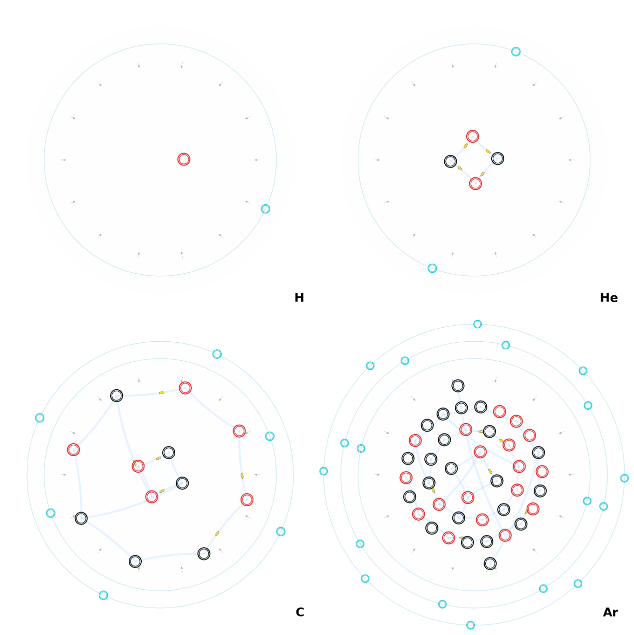
Elements in the diagram:
- Nucleons: red rings = protons, black rings = neutrons;
- Cross-nuclear Corridors: semi-transparent blue bands connect neighboring nucleons and represent near-field settlement channels at nuclear scale; yellow small ovals indicate exchange Wavepackets (gluon appearance);
- Electrons: small cyan rings indicate electronic occupancy in allowed states; pale-cyan concentric circles show the statistical projection of electron shells / Corridor boundaries and do not represent classical circular orbits;
- Element symbol: the lower-right corner labels the element with the English abbreviation, such as H, He, C, or Ar;
- Each panel uses a typical isotope (H-1, He-4, C-12, Ar-40); the shell schematic follows the principal-shell aggregation pattern [2, 8, 18, 32] (for example, Ar = [2,8,8]); the whole figure is only a structural schematic of shells and occupancy, not a substitute for the precise arrangement of quantum states.